Statistical Significance Checker: How to Read Your Results

The badge is green. Your checker returns p = 0.031, the variant is up 1.4 percentage points on the control, and someone has already dropped the screenshot into Slack with the message "ship it Monday?" You have about ninety seconds before the thread makes the decision for you.

Here's the problem with that ninety seconds. The p-value is one row of a table. It answers a narrow question about how unusual your data would look if the variant changed nothing, and it says nothing about whether the change is big enough to bother with, whether it'll hold next month, or whether you looked at the numbers eleven times before today. Read alone, that single number invites the wrong decision.

Read as a set, the same output tells a much more useful story. Walk the fields in the order your checker prints them and each number stops being mysterious.

A statistical significance checker doesn't hand you a verdict. It hands you five or six numbers that only mean something together.

What a Significance Checker Tells You

A statistical significance checker takes raw visitor counts from a control and a variant and returns a p-value, the lift and a confidence interval. Its output is a set of numbers, not a verdict, and it only makes sense when you read the rows as a group.

Say the control converts 12.0% of visitors and the variant converts 13.5%. The checker reports p = 0.03 and a 95% interval for the difference. That's an ordinary Tuesday result, and many teams stop reading at the p-value because it's the field with a threshold attached to it.

Think of the threshold as a smoke detector. You set the sensitivity so the alarm fires in a known share of real fires. When it sounds, it tells you the reading crossed the line. It doesn't tell you how big the fire is, whether it's in this room, or whether someone burnt toast.

Reading the rows in order

Output	What It Means	What It Does Not Mean
p-value	How unusual the data would be if no real difference existed	The probability that the variant works
Absolute lift	The variant's rate minus the control's rate, in percentage points (13.5% minus 12.0% is 1.5 points)	A relative change unless the report says so
Relative lift	The absolute lift divided by the baseline (1.5 points on a 12.0% baseline is +12.5%)	The commercial value of the change on its own
95% confidence interval	The plausible range for the true difference given the data	A guarantee that the true value sits inside the range
Baseline rate	The control group's starting conversion rate	A rate that stays fixed across markets or periods
Sample size per group	The data behind every estimate above	Proof that the result is stable

The first row is where most misreadings begin. A p-value measures how incompatible the observed data are with a specified statistical model. It is not the probability that the null hypothesis is true, and it is not the probability that your result came from chance alone. When a test returns p = 0.03, the accurate description is that data like yours would be relatively unusual under the model you chose. The American Statistical Association statement on p-values puts it plainly: 0.03 is not a 97% probability that the new version works.

That same statement advises against letting a business decision hinge only on whether a p-value crosses a fixed cut-off such as 0.05. It also argues a checker should show the p-value alongside the hypothesis tested, the assumptions, the sample sizes and the estimated effect, rather than returning a binary "significant" or "not significant" label. When your tool gives you the full table, use it. When it gives you only the badge, ask for the rest.

The three numbers to write down

Before you read any verdict, write down three things: the absolute lift, the confidence interval, and the sample size behind both. Those three tell you how big the change is, the range the true value could plausibly sit in, and how much evidence is holding the estimate up. A lift with no interval is a rumour. An interval with no sample size is a guess about a guess.

Everything else in the report is commentary on those three numbers.

How the Checker Calculates Significance

Nothing inside a checker is magic. Every figure it prints comes from four counts and one assumption: that if the variant changed nothing, both groups would be drawn from the same underlying rate. Follow the arithmetic once with a pencil and you'll never be intimidated by the output again.

Here's the path those counts travel, from raw traffic to a p-value.

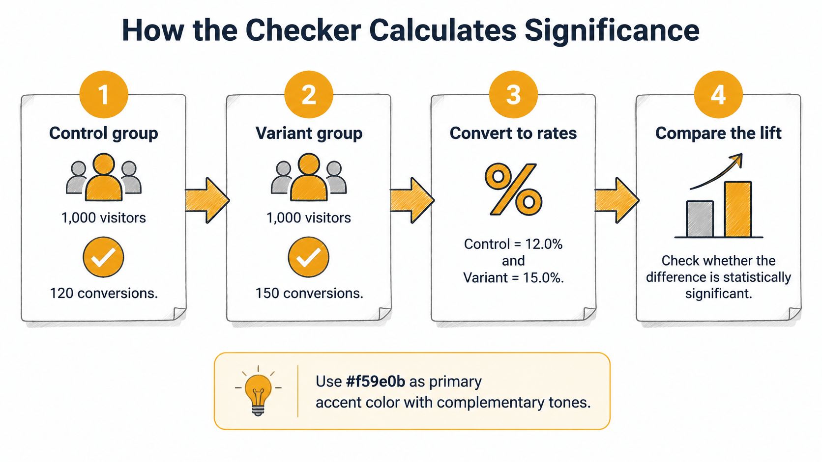
Say the control had 1,000 visitors and 120 conversions, and the variant had 1,000 visitors and 150 conversions.

1. Turn each group into a rate. 120 ÷ 1,000 = 12.0%. 150 ÷ 1,000 = 15.0%. Rates make the groups comparable even when traffic splits unevenly, which raw counts never do.
2. Pool both groups under the no-difference assumption. (120 + 150) ÷ 2,000 = 13.5%. To test "no difference", you need the best estimate of the shared rate the variant would have produced if it changed nothing.
3. Compute the standard error. √(0.135 × 0.865 × (1/1,000 + 1/1,000)) ≈ 0.0153. This converts your counts into the scale on which the gap gets judged, and it shrinks as samples grow. That's why bigger tests can detect smaller lifts.
4. Divide the gap by that error. 0.030 ÷ 0.0153 ≈ 1.96. Expressing the difference in standard errors strips out percentage points and lets a reference table answer the question.
5. Convert to a p-value. A two-sided test maps z ≈ 1.96 to p ≈ 0.05, right on the conventional line. This is the step where a decisive-sounding number turns out to be a coin balanced on its edge.
6. Build the interval around the difference. 3.0 points ± 1.96 × 0.0153 gives roughly 0.01 to 5.99 percentage points. Same information as the p-value, but expressed in the units your stakeholders argue about.

For a single rate rather than a difference, the standard Wald interval takes the form p̂ ± z√[p̂(1−p̂)/n]. NIST Technical Note 2119 works the same example: 120 conversions from 1,000 visitors gives p̂ = 0.12 and an approximate 95% interval of 0.0997 to 0.1403, or about 9.97% to 14.03%. NIST also flags where the normal approximation gets shaky: very small samples, and proportions close to 0% or 100%.

Why the borderline case is not a win

Look at what step five and step six produced together. The p-value landed on the threshold, and the interval's lower bound sits right at zero. Another week of data could push either one across the line in both directions.

That isn't a winner. It's an open question. The right move is to extend the sample or to decide on the size of the lift rather than the badge. One more wrinkle: a one-sided test halves the p-value for identical data, so two checkers can disagree about the same experiment purely because of a radio button you never noticed. Check which one your tool ran before you compare it with anyone else's number.

Practical rule: when the interval's lower bound touches zero, the test hasn't found a difference. It has found a question.

Is the Lift Big Enough to Matter

Significance says nothing about size. A conversion-rate rise from 10.00% to 10.05% can become statistically significant in a very large experiment even though a 0.05-percentage-point gain has almost no commercial value. In the other direction, a rise from 10% to 15% can fail to reach significance in a small, noisy sample and still be worth more than everything else on your roadmap.

The ASA makes both halves of this point in its 2016 statement on statistical significance in The American Statistician: a very small effect produces a small p-value when the sample is large or measurement variability is low, and a large effect produces an unimpressive p-value when the sample is small or measurements are imprecise. The p-value is doing its job in both cases. Your job is a different one.

A worked case where significance wasn't enough

Run a test with a 10.0% control rate and an 11.5% variant rate, about 7,700 visitors per group, and a minimum lift worth shipping of 1.0 percentage point. The absolute lift is 1.5 points, roughly +15% relative. The z-score lands near 3.0 and p ≈ 0.003. Significant by any conventional standard.

Now the interval: 0.52 to 2.48 percentage points. The lower bound of 0.52 sits below the 1.0-point floor your team agreed on. If the true effect were only as large as that lower bound, the change wouldn't cover the engineering time, the QA cycle and the risk of shipping it. Extend the test or keep the baseline. Significant, and still not enough.

An underpowered "not significant" deserves the same care in reverse. It isn't evidence that the two variants perform the same. It's evidence that your test couldn't tell them apart, which is a different claim entirely.

The rule to reuse: write down the smallest lift you would actually ship for before you open the dashboard, then compare the interval's lower bound against that number.

Turning interval position into a decision

Interval Position vs Minimum Lift	Decision	Next Action
Lower bound above the minimum worthwhile lift	Ship the variant	Roll out and keep monitoring the metric
Significant, but the whole interval sits below the minimum lift	Keep the baseline	The gain is too small to justify the effort
Not significant, interval reaches the minimum lift	Inconclusive and underpowered	Retest with a larger sample
Interval includes zero and is wide	Inconclusive	Extend the sample or accept no decision
Upper bound below the minimum lift and narrow	Reject the variant	Stop and test a bigger change

If the case for testing at all still needs making inside your organisation, the argument for the business benefits of A/B testing belongs in front of stakeholders before the next round of debate about a single p-value.

Pitfalls That Create False Winners

A dashboard compares ten keywords across five variants and three audience segments. The highest result may look like a clear winner, but scanning many comparisons raises the chance of finding a false positive by chance.

This is multiplicity: the more comparisons you test, the greater the chance that at least one appears positive even when none has a real effect. For 20 independent tests at a 5% threshold, the probability of at least one false positive is 1 − 0.95²⁰, or 64.2%. That is a probability across the whole set, not the false-positive rate for any one test.

Why twenty tests change the answer

A single test at a 5% threshold has a 5% chance of a false positive under the null hypothesis. Run more independent tests without adjusting the threshold, and the chance of at least one false positive rises.

Comparisons Tested	Chance of At Least One False Positive	Bonferroni Threshold
1	5%	0.05
3	14.3%	0.0167
5	22.6%	0.01
10	40.1%	0.005
20	64.2%	0.0025

The Bonferroni threshold divides the chosen significance threshold by the number of comparisons. With 20 comparisons and a 5% threshold, each test must meet 0.0025. This reduces the chance of even one false positive across the set, though it can also make genuine effects harder to detect.

Bonferroni, false discovery rate, or something simpler

Bonferroni controls the familywise error rate, the chance of at least one false positive across all the comparisons. It can suit decisions where a false win carries a high cost, such as a site-wide redesign.

For screening many keywords or prompts, controlling the false discovery rate may be more appropriate. It limits the expected proportion of false positives among the results flagged as positive, rather than trying to prevent every false positive in the full set.

A simpler safeguard is to name one primary metric before launch. Treat other outcomes, variants, and segments as exploratory: useful for generating questions, but not enough on their own to justify shipping a change. Decide in advance which comparisons belong to the same testing family, then choose a correction that matches the decision's stakes. For help planning the experiment, see sample size considerations for A/B tests.

Before trusting a positive result, ask: How many outcomes, variants, and segments were tested, and was the threshold adjusted for those comparisons?

Checking Results Over Time Without Fooling Yourself

A low-traffic site starts a test on Monday. Someone checks the numbers Tuesday, again Wednesday, again Thursday. On Friday morning the p-value dips to 0.04 and the test is declared won. Traffic is a fraction of what the original plan required, and the variant ships.

That pattern is the single most common way a sound statistical method produces a bad decision. Repeated inspection with a fixed threshold inflates false positives and makes confidence intervals unreliable, even when no real effect exists. Adobe's guide to common A/B testing pitfalls describes the trap directly: one isolated test at a 5% threshold permits a 5% Type I error rate, and that figure describes a test read once, not a test read every morning until it cooperates.

Fixed horizon and sequential analysis are different reports

A fixed-horizon result means the sample size was set in advance and the data were read a single time at the end. The p-value means what the textbook says it means.

A sequential-analysis result means the interim looks were designed in, with boundaries set for each one, so the overall error rate stays where you want it even though you peeked. Both are legitimate. What isn't legitimate is running a fixed-horizon test and then treating an unplanned peek as if it were scheduled.

If a checker doesn't tell you which of those two it produced, you can't read the p-value. That's a reporting gap, not a subtlety.

Write the stopping rule before launch

A good checker should ask you four questions, and you should be able to answer all of them without opening a document:

• Was the sample size fixed in advance? If not, the threshold you're comparing against was never calibrated for your test.
• How often was the data inspected? Two scheduled looks and forty anxious refreshes are different experiments.
• How many variants and metrics were evaluated? This is the multiplicity count, and it decides whether a correction belongs in the report.
• Did the test end early? An early stop is fine when a boundary was designed for it and suspect when it wasn't.

Then do the planning arithmetic. The required sample depends on the baseline rate, the minimum detectable lift and your chosen power, so a team planning for 80% power knows before launch roughly how many visitors each arm needs. Fix the number, then don't touch the dashboard until you reach it.

"We will read this test once, on the date each arm reaches 12,000 visitors, and we will ship only if the lower bound of the 95% interval clears 0.8 percentage points."

One sentence, written before launch, signed off by whoever owns the metric. It settles the argument that would otherwise happen on day four.

Running Significance Checks Across AI Search Benchmarks

A brand shows up in 41 of 120 sampled AI answers, a 34.2% mention rate. Its closest competitor appears in 29 of 120, or 24.2%. Ten percentage points of share of voice, which reads like a rout in a slide deck. Run the two-proportion check and the p-value lands near 0.09. Not significant at any conventional threshold, and the 95% interval is wide enough to contain outcomes from a near-tie to a comfortable lead.

The instinct is to screenshot the 34.2% and take it to the leadership meeting. The better instinct is to ask what would have to change for that number to move.

AI visibility behaves like an experiment with extra noise sources. A brand's mention rate across ChatGPT, Perplexity, Gemini and Google AI Overviews shifts with prompt wording, with the country the question is asked from, and with model updates nobody announced. Sample 120 answers once and you've measured one afternoon of a moving system.

Why the sampling assumption bends

Sampled AI answers aren't fully independent. Five phrasings of the same question can draw on the same retrieved sources and the same model behaviour, so the effective sample is smaller than the count suggests. The interval your checker prints is a guide to the size of the uncertainty, not an exact boundary around the truth.

Treat it the way you'd treat a borderline A/B result: don't call a winner on one reading, and don't call a loss either.

A one-off screenshot of an AI answer is a sample of one. It can start a conversation, but it can't settle one.

LLMrefs was built around that distinction. AI search results are checked in real time, and prompts are continuously checked to ensure statistical significance, so a movement in share of voice gets tested rather than admired. Responses are aggregated across multiple prompts and engines, then normalised and weighted to avoid outliers, which keeps a single dramatic answer from distorting the picture. Customers get stable, comparable visibility metrics instead of one-off screenshots, which is what lets a team track a shift over weeks and know whether it's real.

If you want to see how that kind of benchmark is structured before you commit to one, how AI benchmark rankings work walks through the scoring side.

Confirm Significance Before You Ship a Change

Run this list against any result sitting in front of you. Once the brief exists, each step takes under a minute.

1. Check that the sample size and stopping rule were set before launch. If they were, the p-value is interpretable. If they weren't, treat it as provisional.
2. Name the one primary metric. Then count every other outcome, variant and segment you examined in the same report.
3. Apply a correction when comparisons multiplied. Bonferroni when a false win is expensive, a false discovery rate when you're screening many candidates.
4. Read the absolute lift, the relative lift and the 95% interval together. No number in that set stands alone, and the relative figure is the one most often quoted out of context.
5. Compare the interval's lower bound with the minimum lift worth shipping. That comparison, not the badge, is the decision.
6. Label an underpowered "not significant" as inconclusive. Equal performance is a claim your data has to earn.

The step to take today: write the minimum worthwhile lift and the stopping rule on a single-page brief, rerun the checker with your real visitor counts, and read the interval before you read the p-value.

---

LLMrefs monitors how often your brand appears across AI answer engines like ChatGPT, Perplexity, Gemini and Google AI Overviews, aggregating and weighting responses so each visibility figure comes with the sample behind it, then rechecking significance as new results arrive. Alongside the benchmark dashboards, the free resource tools include an LLMs.txt Generator, a Reddit Threads Finder, an AI Crawlability Checker, a ChatGPT Prompts Database and an AI Content A/B Tester, so you can prepare your content for AI discovery while you measure it. Visit LLMrefs to run your first visibility check and find out whether that gap over your competitor is a real lead or just this week's noise.